There’s an ongoing discussion about attitudes on gray literature (information that has been “published” in some way but has not been peer-reviewed) going on over at ResearchGate. You should check it out.
Tag: research
Quickly access journal PDFs for which UND has a subscription
If you're using Google or another engine to search online for journal articles, seven times out of ten you'll end up at the site where you can get the PDF (via institutional subscription) but you won't be recognized as the institution. This also will happen if you are off-campus. One way to get access is to head back to the UND Libraries site, find the eJournal search, type the name, and then navigate to the right issue. There is a better way.
Take this URL for example. I wound up here after Googling for one of the authors and looking for his email address:
http://jgs.geoscienceworld.org/content/163/4/707.abstract
In order to get that PDF (or see if we even have access), just add the UND proxy to the middle of the URL (bolded for convenience):
http://jgs.geoscienceworld.org.ezproxy.library.und.edu/content/163/4/707.abstract
You'll get bumped to the UND Libraries off-campus login page, and then back to the article page when you've logged in. Now if you click on the PDF link, you'll find out whether we have subscription access (the PDF will open) or not (you'll hit a paywall). This has worked well for me for the past year or so.
Work in progress: genus duration of freshwater mussels in the Hyriidae
My dissertation is dependent on the assumption that people make mistakes in identification and naming of fossil and modern organisms. In particular, I am proposing that certain freshwater mussel genera in the family Hyriidae have supposed taxon ranges that are far longer than they should be, however in order to be taken at least somewhat seriously I need to show that this could be the case and select candidates for further investigation.
The first figure is a simple taxon range diagram for several genera that are agreeably within the Hyriidae. The mean indicators can be ignored. It is apparent that three genera in particular stand out as being long-lived. This could be for a number of reasons: the genera may actually have survived for such long periods of time, certain specimens may have been misidentified, or certain nomenclatural lumping may have occurred inappropriately.
The second figure includes more information. The width of each bean is proportional to the number of occurrences of each taxon through time. Note that the full range of each taxon is not displayed on the second figure because it was produced from age estimates from (in most cases) surrounding stage boundaries.

I will leave it to the reader to determine whether I am on the right track.
Plots were produced in R using the function below, which is being released under the CRAPL. Data is from my personal locality occurrence database, which will become available on the completion of my dissertation.
ranges<-function(locfile,genera=c("Alathyria","Velesunio"),type="box",columns=c("D_no_dissertation_id","genus_bogan","species_source","ref1","age_start_ma","age_end_ma")) {
 # Make sure beanplot is available.
 library("beanplot");
 # Read in the data from a CSV file.
 localities<-read.csv(locfile);
 # List the genera you want.
 # genera<-c("Alathyria","Velesunio");
 # Create a place to store the selections.
 selection<-list();
 start<-list();
 end<-list();
 select<-data.frame();

## For bean plots
 # Grab the whole selection
 select<-subset(localities,localities$genus_bogan %in% genera & localities$age_start_ma!="NA" & localities$age_end_ma!="NA",select=columns);
 # Add mean dates to a data frame.
 select$mean<-ave(select$age_start_ma, select$age_end_ma);
 # Get rid of the unneeded genus names in the subset.
 select$genus_bogan<-factor(select$genus_bogan);

if(type=="box") {
 ## For box plots
 # Loop through the genera
 for (i in 1:length(genera)) {
 # Grab the columns you want.
 selection[[i]]<-subset(localities,localities$genus_bogan==genera[i] & localities$age_start_ma!="NA" & localities$age_end_ma!="NA",select=columns);
 # Sort by column age_start_ma (not needed at the moment).
 # selection[[i]]<-sort(selection[[i]],by=~"age_start_ma")
 # Find the start and end dates.
 start[[i]]<-max(selection[[i]]["age_start_ma"]);
 end[[i]]<-min(selection[[i]]["age_end_ma"]);
 }
 # Make the start and end lists into a matrix...the long way around.
 df<-data.frame(start=unlist(start),end=unlist(end));
 # Transpose the matrix.
 toplot<-t(as.matrix(df));
 # Make a box plot. Don't need to worry about whiskers because there are only two values. The y-axis is reversed.
 boxplot(toplot,names=genera,ylim=rev(range(toplot)),ylab=c("Ma"));
 # Show the data being plotted.
 print(toplot);

 } else if(type=="bean") {

 # Make a bean plot. This is more complicated. The y-axis is reversed.
 beanplot(select$mean~select$genus_bogan, ylim=rev(range(select$mean)), cut=0, log="", names=levels(select$genus_bogan), what=c(0,1,0,0),bw=20,col = c("#CAB2D6", "#33A02C", "#B2DF8A"), border = "#CAB2D6",ylab=c("Ma"));
 }

}
GIS: Raster cell centroids as vector points with GDAL and R
Short intro: I’m using raster data for part of my dissertation, but I’m storing the paleoenvironment data in a database as the latitude and longitude of the center of each grid cell. This lets me query my environment localities, add new ones, and make specific datasets.
Sometimes I take existing maps of other people’s environmental interpretations and digitize them, leaving me with vector polygon data. I need to convert the polygons into the same kind of data I’ve been storing. This is surprisingly hard in both QGIS and GDAL alone, so I finally figured out how to do it in R today courtesy of Simbamangu over at StackExchange.
See the attached images for how things look at each stage.
Below are the general terminal commands, first in GDAL and then R. I will try to add more rationalization and explanation later. My operating system is Mac OS X but these should be modifiable.
GDAL in your terminal
gdal_rasterize -at -where 'freshwater = 1' -a freshwater -ts 360 180 -te -180 -90 180 90 -l "source_layer_name_in_shapefile" "shapefile.shp" "output_raster.tif"
Produces a geoTiff of your input polygons where the attribute ‘freshwater’ is equal to ‘1’. For more detail I invite you to read the GDAL documentation, it’s quite good.
R
To run through a single file:
# load necessary libraries

library(maptools);

library(raster);

library(rgdal);
# Load the raster from a file
r <- raster("rastername.tif")
# Convert to spatial points
p <- as(r, "SpatialPointsDataFrame")
# Set name of column of raster values for later use
names(p)[1]<-"value"
# Get only the values we want (values above zero) in that column
psubset<-subset(p,p$value>0);
# Save as a shapefile (extension appended automatically)
writeSpatialShape(psubset, "outputfile");
You can also loop through a directory:
# load necessary libraries

library(maptools);

library(raster);

library(rgdal);
# Set working directory
setwd("/my/working/directory/");
# list all .tif files in working directory
for (file in dir(pattern="*.tif")) {
r <- raster(file);
p <- as(r, "SpatialPointsDataFrame");
# Set name of column of raster values
names(p)[1]<-"value";
# Get only the values we want (values above zero)
psubset<-subset(p,p$value>0);
# Make a new filename
oldname<-substr(file, start = 1, stop = nchar(file) -4);
newname<-paste(oldname,"pts",sep=" ");
# Make a shapefile
writeSpatialShape(psubset, newname) ;
# Make a CSV file
# Convert to data frame so you can drop extra columns
psubsetdf<-as.data.frame(psubset)
write.table(psubsetdf[,c(2,3)],file=paste(newname,".csv",sep=""),sep=",", row.names=FALSE);
}
Wanted (and some found): Geologic maps (formation contacts) of South America countries, for use in GIS
Here’s a good ol’ plea for help from the scientific community. As my questions to “the scientific community” via Academia.edu have gone unnoticed, I’m posting this out here to see if anyone else searching for the same thing has had any luck. I’m building a GIS (geographic information system) model to determine the possible biogeographic districbution of a genus through time. What I need for this, since the fossils are from South America, is a good geologic map, either of most of the continent or of the countries of Brazil, Argentina, Ecuador, and Peru. Hunting around online hasn’t shown me anything that I want to shell out a bunch of money for, site unseen, and I’m honestly trying to avoid having to scan paper maps and register them (additionally, I haven’t been able to access our worldwide collection of paper geologic maps recently). 1:500,000 or 1:100,000 would be great, but I’d even take 1:1,000,000 at this point. I need something with formational contacts so I can plot possible distributions. So that’s the challenge of the day: have any geologists in South America discovered a good source for this type of material? Would you be willing to share or trade? Drop me an email at one of the addresses on the right sidebar if you can help.
Brazil
UPDATE 2011-08-15: I found (finally) an online version of the Geological Map of Brazil at 1:1,000,000 scale. Unfortunately it is only available in a viewer, broken up into small sections. Anyone know where I can download the full dataset, or at least that data for those sections? UPDATE 2011-08-15 1431: Thanks to Sidney Goveia over at Geosaber, I tracked down the Brazil data to Geobank, so here goes nothing! If you are using a Mac, make sure you extract the contents of the ZIP files using StuffIt Expander (if you have it) rather than Archive Utility, otherwise you don’t end up with a folder.
Peru
UPDATE 2011-08-16: You can download a formation-level geological map of Peru at the 1:1,000,000 scale from INGEMMET – the Instituto Geologico Minero Y Metalurgico. There are a few steps through the online viewer (note: this is the new viewer, so the following steps may not work the same), which may appear in Spanish at first but for some reason decided to reload partway through in English. If you want, you can try to figure out how to turn on the layer under the Map–>Geodatabase menu, but really when that menu comes up you want to click the Download/Descargas folder icon, then select the Geologia layer (SHP icon next to it). It also looks like you can download the data as a KML file for Google Earth. A structural layer (Dominios Estructurales) also looks available, and I checked out the radiometric date layer (Dataciones Radiometricas) as well, which could be useful. You might need to check the projection on the geologic map once you download it. I imported it to QGIS at first and it came up as WGS 84 (probably because of the existing project), but I dug around and figured out that it works as PSAD_1956_UTM_Zone_18S. Need a map key for formation symbols? You can download scans of the paper version of this map from here, one of which has the legend. If the correct map doesn’t come up at that link, click on “Ministerio de Energia y Minas. Instituto de Geologia y Mineria” so see the others. The symbology is different. An alternative large-scale (1:100,000) but low-quality set of maps is available here but will not easily go into GIS.
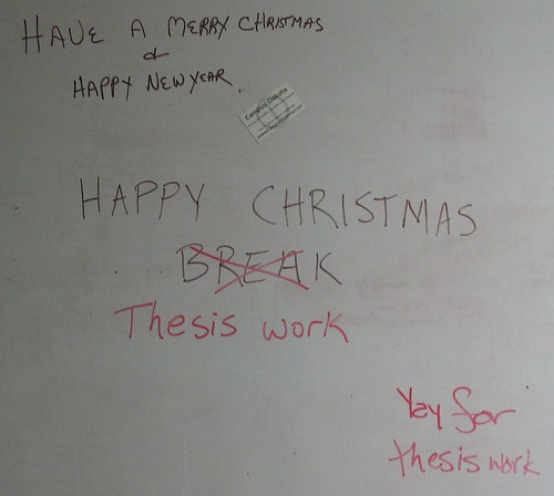
Looking for Inspiration in the End of a Project
It’s the time of year again where I get a break from classes and from being in North Dakota in general, and get to go visit the folks for a few weeks and get some down time. “Down time” being, for a graduate student, the opportunity to get some serious work done without the distractions of classes, advisors, people down the hall, etc.
One of the projects I want to get mostly completed by the time I return in January is to produce two graphics based on literature and museum data concerning my family-level taxon of study. The first of these will be a range chart of the fossil and modern genera (if not species…we’ll see), the second a map showing where all of these taxa can be found. To the commonfolk (i.e., anyone who has never tried this before) this might seem easy, but it’s really going to take a lot of digging through old papers, searching PDFs, and racking up a heck of a list for interlibrary loan next semester. I rediscovered earlier this week that although there may be a lot of information out there on my taxon, some authors didn’t do the best job of organizing what they knew.
Now, you might ask me why I want to use a great deal of my “break” time to do research. The first reason is that I would like to graduate somewhat soon, and the time for, well, wasting time is over. The second reason is something I had to come up with myself for motivational purposes: I want to help people understand things, and to do that I need to be able to make good graphics.
“Infographics” have been the hot new thing for a couple years now, and Tufte will tell you over and over again that you need to include what data are needed and eliminate the stuff that doesn’t matter. I would also argue that things need to be aesthetically pleasing to be educational, something to which I attribute the use of such soothing colors in introductory textbook diagrams. The point I am trying to make is that I need practice in this area, and I might as well practice now, at the beginning of my dissertation, than at the end when all I will want to do is hand-scribble a diagram, scan it, and call it good enough to hand in.
Optimally, my goal is to make these figures (my range diagram and global distribution map) not only good enough to include in a peer-reviewed journal article but good enough to print out as posters and hang on the wall! This is the goal toward which I am striving: I want someone in a similar research area to be able to use my work as a visual reference, and I want someone who has no clue about my research area to be able to look at it and say “oh yeah, I see how this can be useful.” For a great example, see the “Unionoida cum Grano Salis” poster from the Mussel Project.
Goals like “aesthetically pleasing” and “understandable” are intangible and hard to quantify, but that’s also not the entire point–sure, I’ll be happy to get as close as I can, but my real reason is the second motivation I listed above. If I can picture the future where I’m done with the figures, they look good, and I publish them so others can use them, it makes the drudgery of collating occurrence data that much more bearable–and if that is what gets good science done, let’s do it.
Buying PDFs: Commentary
This post was originally a comment on Andy’s post “Buying PDFs: Truth and Consequences” at The Open Paleontologist blog. The text grew too long, so I’m devoting a full post to it, even though it’s a bit rough. The topic is how much we pay for PDFs of published articles, and why this is so disproportionate to physical copies.
People who know me already know what my suggested “solution” is, which is to share as many PDFs with as many people as possible in order to help the publishers reevaluate their prices, however…legality prevents me from supporting taking such action. This is modeled after the philosophy of Downhill Battle: in order to get radio stations to play music beyond the mainstream (paid for by the record companies), we need to bankrupt the record companies, essentially by quitting buying music, or at least music produced by the largest companies who pay the biggest bucks toward keeping their music on the air.
I’m not sure if Andy has a citation for his observation that publishers like Elsevier that continue “to post profits in the midst of the recession”? Having someone play with those numbers a bit would be interesting to do.
This ends up being like gas prices. I get that as a business you get to set your prices as the market will bear, but the strategy of moving more merchandise rather than more expensive merchandise should always be something to consider. How much research do these publishers do as far as sub-fields go? As you say, hospitals can pay top dollar for a single article, but more paleontologists will buy an article if it’s cheaper (especially if they are unaffiliated), will be able to do the research they want, and will be looking for a place to publish.
On that note, I hope people continue to vote with their feet when it comes to open-access vs. closed-access, or even if some journals have slightly lower per-PDF fees. I’ve had the discussion recently about what “high impact” means anymore: nothing. It used to mean that the physical journal was available in more libraries and hence better-read and better-cited, but since everything goes to PDF now, everything (new) is equally available to someone who can do a halfway decent job of searching. This gives us all the freedom to publish in journals with whose practices we agree, rather than who has a wider physical distribution.
Filling
One of my interests is building a PDF library for myself and fellow graduate and undergraduate students. Which means that it’s very hard to pass up PDFs when I come across them on the web. So right now I’m downloading anything I even look at during my research, to keep and to pass along.
This may well fill up my hard drive this semester.
Using ImageJ for what tpsDig does, but on a Mac
If I had discovered this months ago, my thesis would probably be in a much better position right now! I’ve been tied to the PC in my office, rather than being able to go home and watch movies or TV shows while I did my digitizing.
The free program ImageJ is useful for all sorts of things, like processing images for analysis and doing measurements on photographs, but it can also record coordinate (x,y) pairs as an output file, which is perfect for digitizing specimen outlines for later Elliptical Fourier Analysis.
I have been using tpsDig by F. James Rohlf for this, and I’ve never seen an alternative mentioned, probably because most of the other software written for geometric morphometrics is written for DOS and Windows.
Enough blabbering, here’s how to do it:
1. Start ImageJ. Open the image you want to outline.
2. Important! Make sure the coordinate system being used is the same as that in tpsDig (tpsDig places the origin in the lower left, ImageJ in the upper left by default). Select Analyze->Set Measurements…->Invert Y Coordinates.
3. Select the “Polygon Selections” tool on the floating toolbar. [If you’re really good, you could also use the “Freehand Selections” tool and get out scads of numbers.]
4. Outline the object by clicking along the edge of the object. When you close, double click to stop the digitization.
5. Choose File->Save As->XY Coordinates and save your file.
6. You’re done!
To get this to be readable by tpsDig and related software, you will obviously have to add the top three lines that describe the file, the number of landmarks, and the number of curves, as well as the name of the image file as the last line in the file. I don’t have a present need for that, but it’s not too hard to write up an R function (or a terminal script) to add lines (interestingly enough, I’ve been using sed to do this in DOS batch files recently rather than the OS X terminal).
UPDATE: Somewhat annoyingly, ImageJ seems to only open JPG files in RGB colors, not in CMYK. I have no idea why. Luckily, this comes at a time when I am only first starting to realize that CMYK is a more standard color choice than RGB, so most of my files are still in RGB.
If scaling is a factor (it is for me), you can install the Zoom_Exact plugin (near the bottom of the page). Installing this was interesting, but the documentation helped somewhat. What you want to do is:
1. Choose Plugins->New…,
2. Select type “Plugin” and name it “Zoom_Exact”
3. Paste the code into the boz that appears and save it as “Zoom_Exact.java”
4. Restart ImageJ. “Zoom Exact” should appear at the bottom of the Plugins menu.
5. To easily use Zoom Exact, you can map it to a shortcut key with Plugins->Shortcut->Create Shortcut. I have mine mapped to capital “Z” so I can call it up easily when I want to get the scaling right on the screen.
Open-Access Journals
The current annoyance on the VRTPALEO list is the academic publishing industry, who will publish your work in exchange for owning the copyright (meaning that you, as an author, cannot distribute your own work without permission). A simplified but good analogy is made by Scott Aaronson here:
I have an ingenious idea for a company. My company will be in the business of selling computer games. But, unlike other computer game companies, mine will never have to hire a single programmer, game designer, or graphic artist. Instead I’ll simply find people who know how to make games, and ask them to donate their games to me. Naturally, anyone generous enough to donate a game will immediately relinquish all further rights to it. From then on, I alone will be the copyright-holder, distributor, and collector of royalties. This is not to say, however, that I’ll provide no “value-added.” My company will be the one that packages the games in 25-cent cardboard boxes, then resells the boxes for up to $300 apiece.
But why would developers donate their games to me? Because they’ll need my seal of approval. I’ll convince developers that, if a game isn’t distributed by my company, then the game doesn’t “count” — indeed, barely even exists — and all their labor on it has been in vain.
Admittedly, for the scheme to work, my seal of approval will have to mean something. So before putting it on a game, I’ll first send the game out to a team of experts who will test it, debug it, and recommend changes. But will I pay the experts for that service? Not at all: as the final cherry atop my chutzpah sundae, I’ll tell the experts that it’s their professional duty to evaluate, test, and debug my games for free!
We need to figure out a way to exchange information without making people pay exorbitant fees for it, but in the current situation we could be sued for distributing our own work in PDF format. I’m no opponent of paper copies of Journals, but if all you want is a PDF of a work that is peer-reviewed, there’s no reason you should have to pay for it.
EDIT: This person has something to say about it too, with an analogy to the QWERTY keyboard.